Matplotlib is the go-to library for data visualization in Python. Whether you’re working on data science, machine learning, or financial analysis, Matplotlib helps you create clear and informative charts.
Basically you can simply say in short that melt can convert a wide format data to a long format so when you apply plot we get some plot but which is not good so we can make it as a bar chart let’s see kind is equals to bar and you will see that we have the Apple Amazon meta Microsoft so for this also let’s try to print a plot and when we hit shift enter you get little bit better graph because generally this is what happens that in x-axis we have the dates and on the Y we have the prices right Hello friends welcome back to day.
31 of 100 days of hell with python algo trading in previous session we have learned about multi- indexing and we have gone through so many good examples and I hope it’s clear to you and we have also posted the multiple choice questions and the task questions and the mini project so please go through it and you will see that you have good understanding of multi- indexing and now today we will understand the three important concepts of the Python pandas that is melt function PIV table function and the vectorized operations on string.
Because previously we haven’t covered the strings in detail and also the string operations in Python is not that advanced so in pandas we have advanced vectorized operations on string based on the nump array so that it becomes so faster and so efficient so we learn because we also have have to have a good understanding of operations on string because sometimes while data analysis we need to Compare the numbers with the strings let’s say to compare the fundamental analysis and the technical analysis so in that case you will have.


To have a good understanding of the operations on the strings so without further Ado let’s get started so before jumping to the Melt and the PIV table Concepts we have to understand the long versus wide data format so let me tell you the difference if you can see on the screen wide format is where we have a single Row for every data point with multiple columns to hold the values of various attributes means in wi format we have multiple columns right means you can say the number of colums are more than the number of rows.
In the wide data format right whereas in the long format is where for each data point we have as many as rows as the number of attributes and each row contains the value of a particular attributes for a given data point so in the long format we have multiple number of rows right so here we can say the number of rows are significantly larger than the number of columns right this is the long format and this is the wide format it’s like the name also signifies that what is a long and wide format so.
Sometimes it is not necessary that we will be getting the data in a particular format we can get data in Long format also and wide format also so in order to deal with that situation we have to have a good conceptual Clarity on the long data format and the wide data format okay now let’s first visually understand what is the Melt and P table function and then we’ll proceed with the examples so in melt what happens when we have a wide format data let’s say we have multiple number of columns right it.
Can be from hundreds to thousands right the number of columns and the number of rows will be very less right so you can say like this number of columns when we apply the Melt function what will happen this wide format data will get converted to a long format data right so we can say it will become like this the number of rows will be significantly larger than the number of columns right so you can see the definition and the use cases so the Melt function in pandas is used to transform a data frame from a wide.
Format to a long format this can be particularly useful in algorithmic trading for normalizing data making it easier to perform time series analysis or feed it to the machine learning models so in the next session we will understand the time series analysis I would say that is the most important concept of the algo trading because you have to have a good conceptual Clarity on that also you will also learn this time series analysis Concept in the maths also so by applying the Melt function we make it easier to perform.
The time series analysis right then the use cases are normalizing the O LC CV data which we have seen previously open high low close and volume you can refer the video in the I button so when you have o lcv data for multiple assets melt can help consolidate this data into a long format making it easier to analyze or visualize then preparing data for machine learning converting wide format feature data into a long format suitable for training machine learning models so when we start the machine learning.
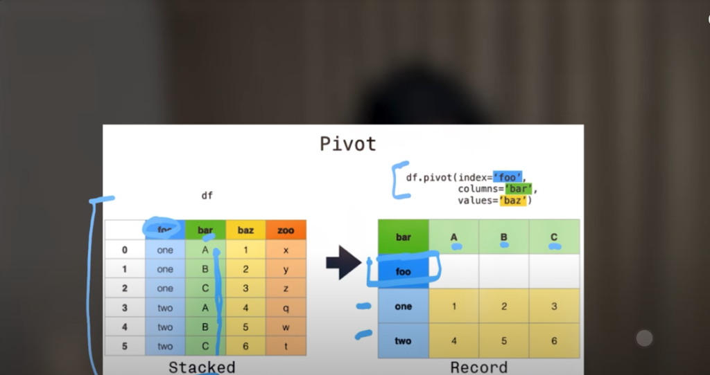
Models you will see that that we are using this melt function a lot right so basically you can simply say in short that melt can convert a wide format data to a long format or you can say the Melt function can melt the wide format to a long format right it’s that simple so the next function is payot I really like a lot this payot function because it is really magical it is awesome to utilize while performing algo trading why because it can transform your data in any form let me show you an example see.
If you can see in the screen we have this table or a data frame right it is stagged so previously we have learned the group by it can perform all those Group by function with a simple pivot command let me show you how let’s say if I want to make this Fu as the index so I just have to provide that DF dop then index is equals to Fu the column name so here you can see that Fu becomes the column name so inside that we have only two unique values so one and two becomes the rows then we can also provide that we want bar column as the columns so you can see here all these unique values becomes the column name again we can also specify that we want values as the bar so in the bar these are the values and these becomes the value of the new modifi data frame don’t worry I’ll show you shortly that how.
We can utilize this in the algo trading but you can imagine that how powerful this function is now let’s understand the use cases of the pavot in the algo trading so a p table in pandas is a powerful data summarization tool it allows you to Aggregate and transform data by changing the structure of a data frame you can completely pivot the data frame to your desired data frame the use cases aggregating trading data summarizing trading data such as average daily returns volumes or other metrics across different time frames or assets creating contingency tables for analyzing the frequency of trading signals or market conditions I’ll show you how don’t worry exactly how we’ll implement this a lot in the upcoming videos we can simply transform any data frame to our desired data frame with the help of the P table function now the last function.
We will understand today is vectorized operations on string and that is the main agenda of the session so what happens in the vectorized string operations let’s say we fetch the data from the the company’s website and it is about the fundamental analysis so generally what happens the data is not structured right we want to analyze and then compare it with the technical analysis so in order to do that we have to structure the data as part our needs so in order to achieve that function we will be using vectorized string operations actually in the core python it becomes so inefficient to perform the string operations so that’s why the pandas came with this vectorized operations and it is based on the numpy array so you know that numpy array is fast and efficient so that’s why we will be using that and again let me show you what is vectorized so let’s say we have a table right 1 2 3 4 so generally what happens in Python if you want to print the square of this list you have to apply four Loop right in the core python but if you apply the numpy operation on this what will happen you just have to give the multiplied by two right and this Square will be applied to all the items in the list and it is known as the vectorized operation a simple operation is applied on all the items in one go and that is known as the vectorized operation.
We’ll learn more about this in the mathematical part don’t worry about that but for now just think that we can apply a single operation in one go so it becomes so faster and efficient and we know that in algo trading we need the speed so now let’s jump to the uh coding part and I’ll show you all these three things the Melt the the pivot table and the vectorized operations okay now let’s start the coding example so let’s build up the base step by step so what we will do first we will create a simple data frame so pd. data frame and inside that we’ll just pass a simple dictionary so let’s say apple and the price is let’s say 100 okay so when I add shift enter it says if using old scal values you must pass an index okay actually you have to pass list here so when you hit shift enter you will see that we have a one row and one column and also we have only single value so if you apply melt on this you will see that this will get converted to this form right it will say variable and value you can also change this I’ll show you later how right now let’s say you have multiple values okay for that what you can do you can like you have BTC with the value let’s say 2,000 then you have the Microsoft with the value 3,000 and let me remove this for now so when you hit shift enter you will get this data frame right and now if you apply melt on this you will see that this wide format data will get converted to the long format data right let me show you again earlier it was this right.
We had uh three columns and when we apply the Melt here uh what will happen it will get converted to like this means the columns will become the rows the values of the rows will also come in the column right now so what is this variable and value actually this is default from the Melt so if you want you can change these names so let’s say the variable name is ticker then if you want to make the value name as the price so you can do that also and when you hit shift enter you will see that it has changed to tier and price now let’s take another example so in which what I’ll do I’ll just copy and paste it here for now I just remove this here what I will do let’s say we have a dictionary in the First Column we have the tickers so let me show you let’s say ticker or tickers and in that we have a list so we can have first Apple then we can have BTC then we can have let’s say Microsoft and we can also have a meta correct I’ll just copy and give a comma here and paste it four times after this we can give let’s say price second column third can be here and it can be let’s say close price just for the sake of example so in price.
We can have let’s say 100 200 and 300 400 right 4 and 300 in ear also you can have and 2021 2 so three 2 and one and in close you can have the close prices so let’s say 11 1 0 then you can have 1 12 0 13 0 or 14 0 so let let me change this make it 220 and 320 and 420 right so now when I shift enter we have to give comma here also here also okay now when you apply melt on this let me apply and when you hit shift enter you will see that everything gets melted all the columns gets melted and you get new two columns which is variable and value but you don’t want to melt all the columns you just want to melt price ear and close and you just want to keep the sticker so for that what you can do you can write here ID and then where and inside that you can pass that you want to keep the ticker right so now when you ship enter okay we have to make this ID Wass not VA so now you will see that tickers is same as previous the Apple BTC Microsoft and meta rest all the three columns gets melted so now.
If you want to make these also customized so what you can do you can give here the the where name is equals to let’s say price and you want to keep this value name as let’s say Capital value right so when you hit shift enter we don’t have to pass this list here you can just give the name in string format so now when you hit ship enter you will see that it has been changed to price and value right so now let’s take some real life example so in which you will learn that how we can implement this so let me show you we import data from the yaho finance first so what I’ll do I’ll just import pandas let’s write it again and we can also import the Y Finance as YF right then we can use yf. download and here we can first do the tickers so tickers we can give let’s say apple and we can also give Amazon we can also give Microsoft and also we can give the meta correct tickers then we can give the start we can start from 24 first gen gen first gen 2 and 24 June 30th correct so now when you hit shift enter you will see that you have the data fetched it is from the live yaho Finance right now so here you can see that we have the multi- index column above we have the close prices high prices low price ohlc data basically and.
Below we have the tickers so if you want to group bu you can apply here the group bu also with a ticker right so when you shift enter you will see that it has been changed and now we have the tickers on the top right you can also bring these values these tickers here in the index so for that you have to stack which we have learned in the previous sessions right so when you stack this you will see that by default we wanted to bring these stickers in the index but instead we got these prices ohlc data here so for that what we can do we can provide the level so it is on the level zero so you will give here level is equals to0 by default what happens the level one index gets stacked so if you want to customize you can just give the level is equals to zero and the top level is zero always and here also the first level is zero and second is level one so now when you hit shift enter you will see that now this will come here and this will go back to their original position so let me hit shift enter and you will see that we have the tickers at the index right or what you can do actually let me just remove this for now and hit shift enter and let’s save this data to a variable named let’s say data okay and I’ll just copy and paste it here and hit shift enter and now what we can do we can apply this that function so I’ll apply stack here so by default we know that.
It will get stack let’s see that right but we wanted the stickers so we have to apply level level is equals to zero correct so here we are getting the warning future warning So to avoid this for now what you can do you can write here future stack is equals to true and this warning will go away for now okay that warning was because it has been replicated and it might possible that you might get error in the future so for that always try to use the updated functions so here we have just removed temporarily that warning and now what we can do we will reset the index okay so reset index and when we apply this by default what will happen the level zero index will be reseted but we want the level one index so here we can also provide the level is equals to one and you will see that the level one which is meta Amazon Microsoft has been reseted right now I guess we are good to go for the Melt so I’ll again reassign to data and I’ll print it here now our main goal is to melt this means we want to keep the date and ticker here and rest all the values we want to like convert from The Columns to rows right so if you apply melt here you will see that by.

Default everything gets melted but we don’t want that we want to keep the date and ticker there so what I will do now I have shown you earlier that melt and here you can give ID where and inside that you can pass a list so we want to keep date as it is and also we want to keep ticker as it is so now when you shift enter you will see that it says the following ID where value are not present in the data frame let me show you the issue here is that this date is the index right now so for that what you can going to do you can apply.
The reset index here and you will get the default Index right now that date becomes the column so now if you apply the Melt what will happen these date and ticker columns will remain as it is and you will see that date and ticker is same right and this price and value is new so for that what you can do you can also pass here the V name is equals to you can say and also the value you can make it as the capital so what I will do here value name is equals to Value capital V value right now when you H shift enter what will happen you will get here the Matrix and the value now again in this variable what you wanted like which column should be here right so for that what you can do you can just write here uh so let me show you again uh what we will do I’ll just uh first print the data here and let me show you so this was the original data right so in the value of variable what you want o h l c v and the last Adent close so for that what you can do you can simply go here and write value vs and then you can pass these values right uh all these so open high low close and volume so.
I’ll go here I’ll pass here and I’ll make this a string this also let give comma and this also and a comma here also comma and the last one is volume and let’s so now what will happen you will see that you get the modified uh data frame so for that you have to remove this and see the modifi data frame and this is your modified data frame so here we have a date then tickers then the matrices that is open high low Clos and volume then the value so that’s how you can use the Melt function uh I tried my best to show you if you still have any doubt please let me know we can discuss further on this right okay now let’s understand the P table it is really very very useful function for everyone okay so what we’ll do we’ll take the real world data set so if you remember we have F the data from the yo Finance on the initial part of the session uh here we know that we store the data in that data variable right so what I’ll do I’ll use the same data here so when I print this we have this this one correct so in index we have date and on the columns we have the ticker O lcv Let’s also check the info you’ll get more details so the ticker here is the object rest all are float 64 and the volume is integer 64 right and also.
We have the index as the date time index don’t worry we will understand this date time index in the next session because it is one of the most important topic on the Alo trading you have to understand this thoroughly so that’s why I’ll take whole session for this daytime Index right so now what we can do let me show you that where we can use the PIV table so let’s say if I want to apply a group biome this so what I can do I can apply a simple group biome ticker right then what we can do we can uh find the mean of open price right so mean and you will get this value correct and if you also want to uh Group by with the date so then what you can do you can like group by with the ticker and date and then you can find the mean so you will get mean of every day for each scker okay now let me show you that you can make this series as the data frame which we have seen previously that with the unstack you can make this 1D data to the 2D data frame so for that you will be using unstack and by applying unstack what will happen here that this level one index will get to the column names so it will become the column names and now when I hit shift enter you will see that we have only four rows and 11 n columns right so we have done this with the help of group by but same thing.
We can achieve with the p table let me show you how let’s say if I apply P table not DF data data P table right and here you can pass the index so here the index is ticker so you can give index as the ticker right so when you hit ship enter you will get this value right the index is tickers and rest by default it calculates the uh mean value right so now we want the 11 n columns so what we can do at the columns we can give here the value as like columns I want date right so when I ship enter you will see that now we have four rows but 714 columns so what happened here it has calculated for every Matrix like the Addison close open high low close and volume but we want only for the open so in the value the cell values these values you can provide here that you want value as the open right and now when you hit shift enter you will see that we have exactly the same result with the group buy so when you have like a big group by statement so instead of using Group by you can use p table so it’s like a straightforward and very quicker way to transform your data from 1D to 2D or your desired values right now let me uh show you something uh I’ll just copy and paste it here and if I apply aggregate function here and I apply mean you will see that it has exactly the same value right so by default it applies the main function now what you can do let’s say here we only use the open right the open price.
If you want to apply pay table in all the columns so for that what you can do you can just copy from here and paste it here just remove this values so it will apply on everything so when you hit shift enter you will see that now we have the adjacent close also we have the volume also and the remaining are hidden so you can’t see them but here you can see the number of columns that is 714 right so you can also apply different aggregate function on each Matrix like on close you want to apply something else on volume you want to apply something else let me show you how so what you can do here you can pass a dictionary here and you can give like on open you want to apply mean so I’ll just make it a string mean then next is let’s say we have what we have here data let me print it here so here we have open high low close and volume so what I’ll do here on open we applied mean then on high we can apply let’s say Max so max then on close you can apply minimum and on volume you can apply the sum right so on volume you can apply the sum right so now when you hit shift enter you will see that we have separate aggregate function on every Matrix like the Open high low close and volume so that’s how you can use this and you can also make it multi-dimensional so let me show you how I’ll just copy and paste this here and now let’s say you want to make the multi-index so what you can do here you can just pass a list here and along with the ticker you can also give another column let’s say you want to make date as the index and now when you hit shift enter you will see that.
We have a multi-index data frame right first we have ticker then and we have the date if you want you can make date as the level zero index so you can just reverse the positions the index positions And now when you hit shift enter you will see that first we have date then we have ticker right let’s make it again so it looks nice now the NN values means at that place we don’t have any value so that’s why we are getting the NN next we have is the margins right so in margin what happens let me show you first so what I’ll do I’ll just copy and paste the above here and paste it here and I’ll remove everything from here and I’ll just keep one aggregate function that is sum and I’ll also remove this column and I’ll keep here let’s say volume in column and I’ll remove from here the date also okay now when I Shi enter I’ll get this value right so if we apply the margins here and we make it true you will see that we get the sum of all the columns right you can see here and also here sum of every value in the row right if you remove the column you will get only the sum of columns you can see here we have all as the row and if you make here the column then you will also get the margins in the rows you can see here so that’s how you can use the margins it is sometime it is useful right now let’s move further and uh let’s float some graphs right.
It is now interesting right because when we have graphs it becomes really interesting so what we will do let’s again print the main data frame that is data and let’s say we want to apply pivot table on this and we want to make index as the tickers right so let’s apply the plot here so when you apply plot we get some plot but which is not good so we can make it as a bar chart let’s see kind is equals to bar and you will see that we have the Apple Amazon meta Microsoft and in the prices we have this but you can make it a little bit more like visible so for that what you can do you can make let’s first print this so I’ll just keep it here this is just for illustration okay you have to like practice yourself a lot on this so let’s try that uh I want uh column as the date right or let’s make date as the index and columns as the ticker as the ticker and when we hit shift enter we get something like this so we can also make values as the open prices right or if you want we can make make it close also and you will get this right so for this also let’s try to print a plot and when we hit shift enter we get little bit better graph because generally this is what happens on the x-axis we have the uh datee and on the Y we have the prices so you can see here a nice and beautiful plot and if you want to make it something let’s say a kind you can make it bar also.
If it makes sense right you can see here but it doesn’t make sense so it’s not a good idea to make it as a bar plot you can also make it a pie chart right but it says it is saying some error so let’s not do that and make it a simple chart so now I think you are able to see that this is really very powerful and you can do many amazing things with the help of fas and the so many amazing functions right so in the next session we will understand the vectorized operations on the strings and again a very important part that is time series analysis that is the most important I would say and then we’ll proceed with the visualization part in which we’ll we’ll try to plot some interesting stuffs then we will proceed with the core algo trading Concepts right in which we’ll learn a lot of theory and also we’ll Implement all those on the live markets so with that being said this was it for the session I hope you liked it and if you liked it please let us know and if you don’t like also please let us know so we’ll see you in the next session until then bye-bye take care have a nice day.
Watch this Day 31 video tutorial
Day 31: Pivot Table and Melt in Pandas